Mobile Robot Formation Control

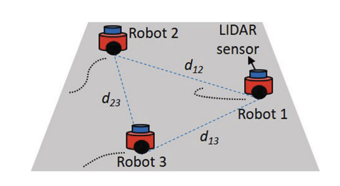
Project Overview

This project investigates the design, analysis, and implementation of distributed formation control laws for a multi-robot system. We tackle the problem from two complementary perspectives: a classical model-based distance-based control approach that provides analytical stability guarantees, and an end-to-end learning-based decentralized control approach that operates directly on raw LiDAR scans without requiring inter-agent communication.

Unlike position-based or displacement-based formation controls, distance-based control does not require absolute coordinate sensing or orientation alignment between robots. Instead, the desired geometric shape is defined solely by inter-agent distances, which makes it highly suitable for vision-based or GPS-denied indoor environments. However, distance-based formation control imposes a strict graph rigidity requirement to ensure stable convergence.

Model-Based Distance-Based Formation Control

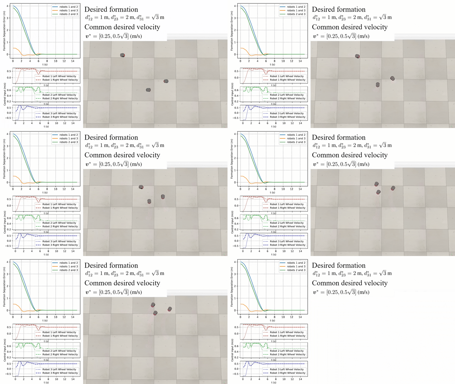
We first design an analytical state-feedback control law for a three-robot team with an undirected interaction graph. The target geometric configuration is represented by desired distances $d^*_{ij} = d^*_{ji} > 0$ for each edge $(i, j) \in \mathcal{E}$.

1. Kinematics and Separation Error

Assuming a group of three agents operating under the single-integrator kinematic model:

$$\dot{p}_i = v_i, \quad i \in \mathcal{V} = \{1, 2, 3\}$$

where $p_i = [x_i, y_i]^T \in \mathbb{R}^2$ represents the position, and $v_i \in \mathbb{R}^2$ represents the velocity control command. The inter-agent relative displacement is $\tilde{p}_{ij} \triangleq p_i - p_j$. The formation separation error is:

$$e_{ij} = \|\tilde{p}_{ij}\| - d^*_{ij}, \quad \forall (i, j) \in \mathcal{E}$$

2. Gradient-Descent Control Law with Collision Avoidance

To drive the separation error to zero while guaranteeing safety, we formulate a gradient-descent control law derived from a candidate Lyapunov potential function $\gamma_{ij}(\|\tilde{p}_{ij}\|^2)$ that approaches infinity if agents get too close:

$$\gamma_{ij}(\|\tilde{p}_{ij}\|^2) = \frac{K_g}{2}\frac{(\|\tilde{p}_{ij}\|^2 - d^{*2}_{ij})^2}{\|\tilde{p}_{ij}\|^2}$$

where $K_g > 0$ is a positive controller gain. Taking the partial derivative with respect to $\beta_{ij} \triangleq \|\tilde{p}_{ij}\|^2$, we obtain:

$$\rho_{ij} = \frac{\partial \gamma_{ij}(\beta_{ij})}{\partial \beta_{ij}} = K_g \frac{\|\tilde{p}_{ij}\|^4 - d^{*4}_{ij}}{\|\tilde{p}_{ij}\|^4}$$

The distributed gradient controller for each agent driving the system toward the desired formation with a common group velocity $v^* \in \mathbb{R}^2$ is expressed as:

$$v_i = v^* - \sum_{j \in \mathcal{N}_i} \rho_{ij} (p_i - p_j)$$

Under LaSalle’s Invariance Principle, if the initial positions of the three robots are non-collinear (i.e., $\det[\tilde{p}_{12}(0), \tilde{p}_{23}(0)] \neq 0$), the geometric formation asymptotically converges to the desired target $\mathcal{B} = \{ \tilde{p} : \|\tilde{p}_{ij}\| = d^*_{ij} \}$, and each robot’s velocity converges to $v^*$.

3. Nonholonomic Coordinate Transformation

To deploy this algorithm on physical differential-drive robots (such as the Pioneer P3-DX), we apply a hand-position coordinate transformation. The reference point $p_i = [x_i, y_i]^T$ is placed a distance $c = l/2$ (half the track width $l$) ahead of the wheel axle midpoint $q_i = [q_{xi}, q_{yi}]^T$ along the robot orientation $\theta_i$:

$$\begin{bmatrix} x_i \\ y_i \end{bmatrix} = \begin{bmatrix} q_{xi} + c\cos\theta_i \\ q_{yi} + c\sin\theta_i \end{bmatrix}$$

Differentiating this transformation yields the decoupled single-integrator system $\dot{p}_i = [v_{xi}, v_{yi}]^T$, which can be mapped directly to target left and right wheel velocities ($v'_{Li}, v'_{Ri}$):

$$\begin{bmatrix} v'_{Li} \\ v'_{Ri} \end{bmatrix} = \begin{bmatrix} \sin\theta_i + \frac{l}{2c}\cos\theta_i & \sin\theta_i - \frac{l}{2c}\cos\theta_i \\ -\sin\theta_i + \frac{l}{2c}\cos\theta_i & \sin\theta_i + \frac{l}{2c}\cos\theta_i \end{bmatrix} \begin{bmatrix} v_{xi} \\ v_{yi} \end{bmatrix}$$

4. Curvature Preservation under Actuator Saturation

To handle hardware limits where individual wheel speeds are capped at $v_m = 0.7\text{ m/s}$, the command velocities undergo a down-scaling transformation:

$$\begin{bmatrix} v_{Li} \\ v_{Ri} \end{bmatrix} = \min\left\{v_m, \frac{v_m}{\max(|v'_{Li}|, |v'_{Ri}|)}\right\} \begin{bmatrix} v'_{Li} \\ v'_{Ri} \end{bmatrix}$$

Since the scaling is applied equally to both wheels, the radius of curvature $R = \frac{2(v_{Li} - v_{Ri})}{l(v_{Li} + v_{Ri})}$ is mathematically preserved ($R' = R$), ensuring that the physical robot trajectory remains undistorted despite actuator saturation.

Learning-Based Decentralized DNN Integration

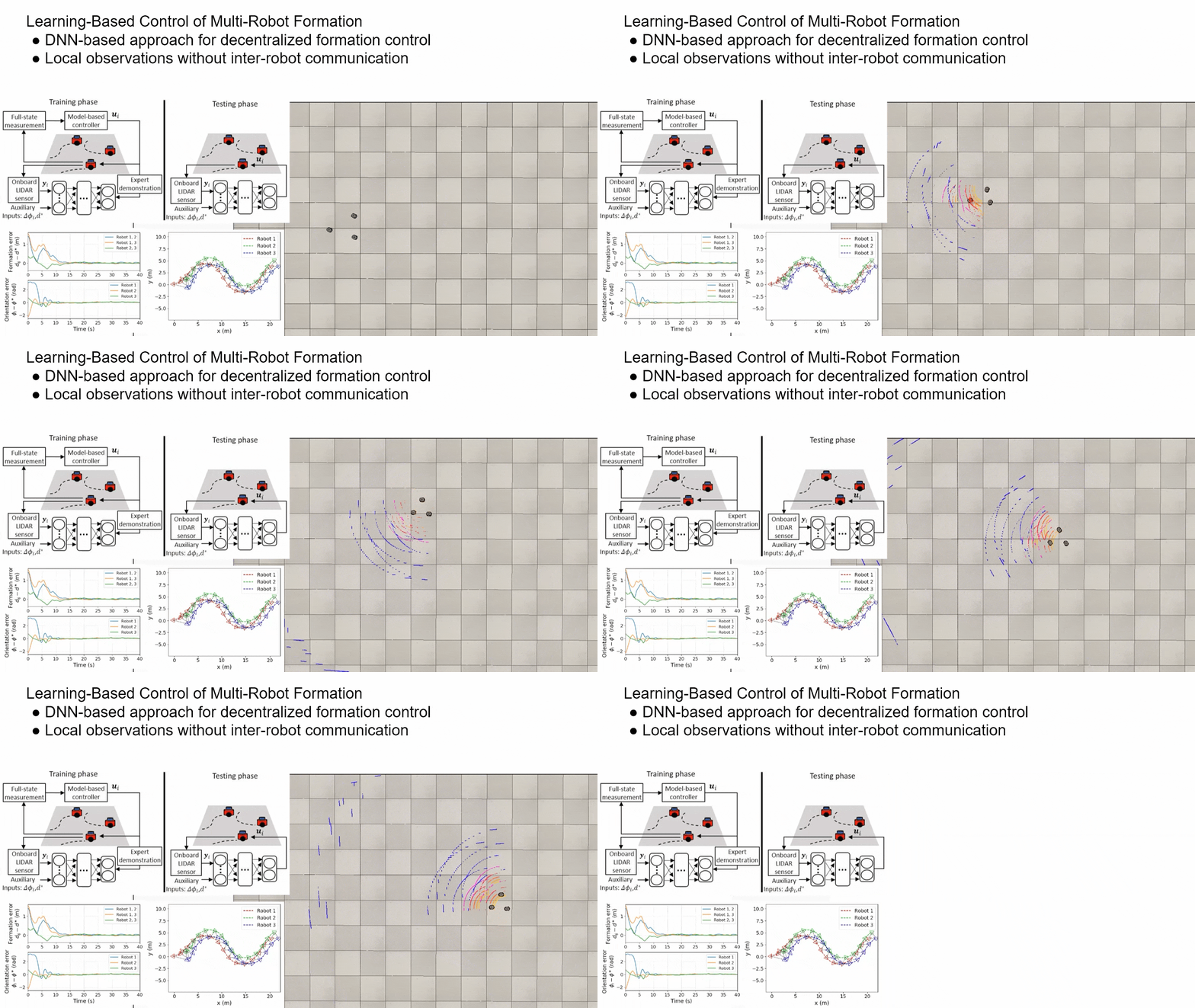
Traditional model-based methods rely on communication to exchange relative position measurements and are vulnerable to model uncertainties or sensor calibration drift. To resolve this, we present an end-to-end learning-based control policy that maps a robot’s local raw LiDAR scans directly to motor commands.

1. Control Policy Formulation

The decentralized control policy is modeled as:

$$\hat{u}_i = F(y_i, \Delta\phi_i, d^*)$$

where:

• $y_i \in \mathbb{R}^{50\times50\times1}$ is a 2D grayscale occupancy map representing the local LiDAR scan in a $5\text{m} \times 5\text{m}$ square centered at robot $i$, with a spatial resolution of $0.1\text{ m/pixel}$.
• $\Delta\phi_i = \phi_i - \phi^*$ represents the orientation error between the robot’s current heading $\phi_i$ and the desired target heading $\phi^*$.
• $d^*$ is the desired inter-robot distance.
• $\hat{u}_i = [\hat{u}_{il}, \hat{u}_{ir}]^T$ represents the normalized left and right wheel speed commands.

2. Deep Neural Network Architecture

The control policy $F(\cdot)$ is parameterized by a deep neural network consisting of a Convolutional Neural Network (CNN) feature extractor and a Fully-Connected (FC) decision network:

• CNN Layers (Feature Extraction):
  • Conv 1: 32 filters, $8\times8$ filter size, stride 4, outputs $12\times12\times32$ feature maps with ReLU.
  • Conv 2: 16 filters, $4\times4$ filter size, stride 2, outputs $5\times5\times16$ feature maps with ReLU.
  • Conv 3: 16 filters, $3\times3$ filter size, stride 1, outputs $3\times3\times16$ feature maps with ReLU.
  • Flattened into a 144-dimensional feature vector.
• FC Layers (Control Output):
  • Hidden Layer 1: 32 hidden units, fused with the auxiliary scalar inputs ($\Delta\phi_i$, $d^*$), activated via ReLU.
  • Output Layer: 2 units with linear activation, yielding normalized motor commands $\hat{u}_i$.

3. Centralized Training and Online Deployment

We generated 110,160 training samples from V-REP expert demonstrations using the model-based controller. The parameters $\theta$ of the DNN were optimized by minimizing the Euclidean loss:

$$\mathcal{L}(\theta) = \frac{1}{N_B} \sum_{j=1}^{N_B} \|\hat{u}_j - u_j\|^2$$

using the Adam optimizer (learning rate $\eta_0 = 10^{-4}$, mini-batch size 32) over 500 epochs.

During online testing, the trained network runs decentralized on each robot. It computes motor control commands $u_i = K \hat{u}_i$ in real time (taking just $2.1\text{ ms}$ of inference time). This approach completely eliminates the need for inter-robot communication and hand-engineered perception pipelines, achieving a 96% success rate within a 10% error tolerance.

Methodology Comparative Analysis

A comparison between the two approaches highlights a trade-off between mathematical stability guarantees and operational independence in complex environments:

Dimension	Model-Based Method (CCDC 2019)	Learning-Based Method (AIM 2019)
Model Dependency	High (Requires precise kinematics and transformation matrices)	Zero (Purely data-driven policy learning)
Sensing Requirements	Relative position vectors (requires explicit coordinates)	Grayscale local occupancy maps (raw LiDAR scans)
Communication	Necessary (Inter-robot communication to exchange states)	Zero (Communication-free local sensing)
Computation Cost	Minimal (Analytical control laws, low CPU overhead)	$2.1\text{ ms}$ per step (Requires neural network inference)
Robustness	Vulnerable to model uncertainties and calibration drift	Highly robust to model errors (inherent in data representation)
Stability Proof	Rigorously proven using LaSalle’s Invariance Principle	Empirical validation (No analytical closed-loop proof)

---

项目概览

本项目设计、分析并实现了多机器人系统的分布式编队控制算法。我们从两个互补的维度对该问题进行了研究：一类是经典的基于模型的距离编队控制方法，提供了严格的解析稳定性证明；另一类是基于去中心化深度神经网络 (DNN) 的端到端学习控制方法，可直接处理原始激光雷达 (LiDAR) 测距数据，且不需要机器人之间进行任何数据通信。

与基于位置 (Position-based) 或基于位移 (Displacement-based) 的编队方法不同，基于距离的编队控制不需要机器人感知全局绝对坐标或对齐局部坐标系朝向。整个期望编队形状仅通过机器人间的相对距离来定义，这使其在基于视觉导航或无 GPS 信号的室内环境中具有极高实用价值。然而，基于距离的编队控制在图拓扑上必须满足刚性 (Rigidity) 要求，以确保系统的稳定收敛。

基于模型的距离编队控制

我们首先针对具有无向交互拓扑的三机器人系统，设计了状态反馈编队控制算法。目标几何外形由每条边 $(i, j) \in \mathcal{E}$ 的期望距离 $d^*_{ij} = d^*_{ji} > 0$ 来定义。

1. 运动学与编队偏差

假定三机器人系统满足单积分器 (Single-integrator) 运动学模型：

$$\dot{p}_i = v_i, \quad i \in \mathcal{V} = \{1, 2, 3\}$$

其中 $p_i = [x_i, y_i]^T \in \mathbb{R}^2$ 表示位置坐标， $v_i \in \mathbb{R}^2$ 为速度控制指令。机器人间的相对位移定义为 $\tilde{p}_{ij} \triangleq p_i - p_j$。则编队的分离偏差为：

$$e_{ij} = \|\tilde{p}_{ij}\| - d^*_{ij}, \quad \forall (i, j) \in \mathcal{E}$$

2. 带避障特性的梯度下降控制律

为了在消除编队分离偏差的同时确保行进过程的安全，我们设计了一个基于李雅普诺夫候选势函数 $\gamma_{ij}(\|\tilde{p}_{ij}\|^2)$ 的梯度控制律。当机器人间距趋于零时，该势函数将趋于无穷大，从而实现物理避障：

$$\gamma_{ij}(\|\tilde{p}_{ij}\|^2) = \frac{K_g}{2}\frac{(\|\tilde{p}_{ij}\|^2 - d^{*2}_{ij})^2}{\|\tilde{p}_{ij}\|^2}$$

其中 $K_g > 0$ 为正的控制器增益。对自变量 $\beta_{ij} \triangleq \|\tilde{p}_{ij}\|^2$ 求偏导可得：

$$\rho_{ij} = \frac{\partial \gamma_{ij}(\beta_{ij})}{\partial \beta_{ij}} = K_g \frac{\|\tilde{p}_{ij}\|^4 - d^{*4}_{ij}}{\|\tilde{p}_{ij}\|^4}$$

为了引导多机器人系统以共同的编队速度 $v^* \in \mathbb{R}^2$ 收敛至期望几何形状，分布式梯度控制器最终被设计为：

$$v_i = v^* - \sum_{j \in \mathcal{N}_i} \rho_{ij} (p_i - p_j)$$

应用 LaSalle 不变原理 (LaSalle’s Invariance Principle) 可以证明，如果三机器人的初始位置不共线（即满足行列式条件 $\det[\tilde{p}_{12}(0), \tilde{p}_{23}(0)] \neq 0$），则该几何编队将渐近稳定收敛至目标流形 $\mathcal{B} = \{ \tilde{p} : \|\tilde{p}_{ij}\| = d^*_{ij} \}$，且各机器人速度将收敛到 $v^*$。

3. 非圆约束坐标变换 (手位置技术)

为了将上述算法应用于差速驱动机器人平台 (如 Pioneer P3-DX)，我们引入了非圆约束的手位置变换。控制参考点 $p_i = [x_i, y_i]^T$ 设在驱动轮轴中心 $q_i = [q_{xi}, q_{yi}]^T$ 沿机器人朝向角 $\theta_i$ 前方 $c = l/2$ 处（其中 $l$ 为轮距）：

$$\begin{bmatrix} x_i \\ y_i \end{bmatrix} = \begin{bmatrix} q_{xi} + c\cos\theta_i \\ q_{yi} + c\sin\theta_i \end{bmatrix}$$

对该式求导可将非holonomic差速驱动运动学转化为完全解耦的单积分器系统 $\dot{p}_i = [v_{xi}, v_{yi}]^T$，并可直接解算出左右轮的目标驱动线速度 ($v'_{Li}, v'_{Ri}$):

$$\begin{bmatrix} v'_{Li} \\ v'_{Ri} \end{bmatrix} = \begin{bmatrix} \sin\theta_i + \frac{l}{2c}\cos\theta_i & \sin\theta_i - \frac{l}{2c}\cos\theta_i \\ -\sin\theta_i + \frac{l}{2c}\cos\theta_i & \sin\theta_i + \frac{l}{2c}\cos\theta_i \end{bmatrix} \begin{bmatrix} v_{xi} \\ v_{yi} \end{bmatrix}$$

4. 执行器饱和下的曲率保持

为了应对执行器物理限制（单轮最高速度限制为 $v_m = 0.7\text{ m/s}$），控制器对指令速度进行等比例缩放变换：

$$\begin{bmatrix} v_{Li} \\ v_{Ri} \end{bmatrix} = \min\left\{v_m, \frac{v_m}{\max(|v'_{Li}|, |v'_{Ri}|)}\right\} \begin{bmatrix} v'_{Li} \\ v'_{Ri} \end{bmatrix}$$

由于缩放是对左右轮速度同比例进行的，机器人的轨迹曲率半径 $R = \frac{2(v_{Li} - v_{Ri})}{l(v_{Li} + v_{Ri})}$ 在数学上保持完全不变 ($R' = R$)。这意味着即使存在执行器饱和，物理运动轨迹也不会发生形状畸变。

去中心化 DNN 编队控制集成

传统的基于模型的方法必须依赖传感器数据的显式坐标计算，容易受到模型参数不确定性及传感器校准漂移的影响。为此，我们设计了一种基于深度神经网络 (DNN) 的端到端去中心化控制律，直接将机器人的局部原始 LiDAR 激光雷达测距数据映射为电机转速指令。

1. 控制策略公式化

去中心化控制策略表示为：

$$\hat{u}_i = F(y_i, \Delta\phi_i, d^{*})$$

其中：

• $y_i \in \mathbb{R}^{50\times50\times1}$ 是以机器人 $i$ 为中心、 $5\text{m} \times 5\text{m}$ 范围内的 2D 局部占用栅格图 (Occupancy Map)，由车载激光雷达扫描生成，空间分辨率为 $0.1\text{ m/pixel}$。
• $\Delta\phi_i = \phi_i - \phi^*$ 表示机器人当前朝向 $\phi_i$ 与目标朝向 $\phi^*$ 之间的角度偏差。
• $d^*$ 是期望的机器人间编队距离。
• $\hat{u}_i = [\hat{u}_{il}, \hat{u}_{ir}]^T$ 是归一化后的左右轮电机控制指令。

2. 深度神经网络架构

控制策略 $F(\cdot)$ 采用由卷积神经网络 (CNN) 特征提取器与全连接 (FC) 决策网络组合而成的 DNN 架构：

• CNN 卷积层 (特征提取):
  • 第 1 卷积层 (Conv 1): 32个滤波器，卷积核尺寸为 $8\times8$，步长 4，利用 ReLU 激活生成 $12\times12\times32$ 特征图。
  • 第 2 卷积层 (Conv 2): 16个滤波器，卷积核尺寸为 $4\times4$，步长 2，利用 ReLU 激活生成 $5\times5\times16$ 特征图。
  • 第 3 卷积层 (Conv 3): 16个滤波器，卷积核尺寸为 $3\times3$，步长 1，利用 ReLU 激活生成 $3\times3\times16$ 特征图。
  • 最终展平为一个 144维的特征向量。
• FC 全连接层 (控制决策):
  • 第 1 全连接层 (Hidden 1): 32个隐层节点，与辅助标量输入 ($\Delta\phi_i$ 及 $d^*$) 拼接融合，通过 ReLU 激活。
  • 输出层: 2个输出节点，采用线性激活，直接输出左右轮的归一化线速度控制量 $\hat{u}_i$。

3. 集中式训练与在线分布式部署

在 V-REP 仿真环境中，利用上述基于模型的专家控制器进行示范数据采集，共积累了 110,160 个样本数据。通过最小化神经网络输出 $\hat{u}_j$ 与专家动作 $u_j$ 之间的欧氏损失函数来优化权重参数 $\theta$：

$$\mathcal{L}(\theta) = \frac{1}{N_B} \sum_{j=1}^{N_B} \|\hat{u}_j - u_j\|^2$$

采用 Adam 优化器 (初始学习率 $\eta_0 = 10^{-4}$，批大小为 32) 进行了 500 个 Epoch 的集中式训练。

在实际测试阶段，训练完成的网络参数固化并在各机器人上以完全分布式运行。每次控制循环的神经网络前向计算仅需 $2.1\text{ ms}$ 的推理时间。这种方法彻底避免了传统控制中繁杂的障碍物检测、状态识别 and 坐标计算等特征手工工程，在 10% 误差容忍下实现了 96% 的编队成功收敛率。

编队控制方法对比

经典控制理论方法与新兴学习算法的对比，展示了数学严谨稳定性与未知环境自适应能力之间的平衡：

对比维度	基于模型的方法 (CCDC 2019)	基于深度学习的方法 (AIM 2019)
模型依赖性	高（严重依赖机器人运动学模型与参数转换矩阵）	无（纯粹基于数据的策略模型训练）
感知需求	需要相对位置矢量（必须进行显式的邻居相对坐标测量）	仅需局部占用栅格图（基于车载激光雷达原始数据扫描）
通信成本	必须（需要跨机器人实时通信以共享状态/坐标）	无（零通信开销，完全基于局部自主观测）
计算复杂度	极低（解析级控制律，几乎不消耗 CPU 资源）	$2.1\text{ ms}$ 前向计算（需要微型车载 GPU/CPU 推理）
自适应与鲁棒性	对参数漂移、动态摩擦和传感器校准误差较为敏感	对模型不确定性具备极强鲁棒性（不确定性被直接固化于特征表示中）
数学稳定性证明	基于 LaSalle 不变原理提供了严格的解析收敛性证明	依赖大规模实地与仿真统计验证（目前缺乏闭环解析证明）